Polynomial Regression — Gradient Descent from Scratch

No libraries, no problem

​ Photo by Jonny Caspari on Unsplash

Gradient descent is an important algorithm to understand, as it underpins many of the more advanced algorithms used in Machine Learning and Deep Learning. Getting to grips with the inner workings of gradient descent will therefore be of great benefit to anyone who plans on exploring ML algorithms further.

The best way to learn is by doing, so in this article I will be walking through the steps of how the gradient descent process works, without using ML libraries such as scikit-learn for example. In day-to-day work, it is of course quicker and neater to make use of such libraries, but regarding the learning process I have found the exercise of implementing by hand to be invaluable for this particular algorithm.

Goal of Gradient Descent — First Steps

The goal of gradient descent is to minimize the error of a model’s prediction, relative to the original data. In this article’s context, we will be looking at a second-degree polynomial model, also known as a quadratic equation:

Second degree polynomials tend to look something like this, when plotted:

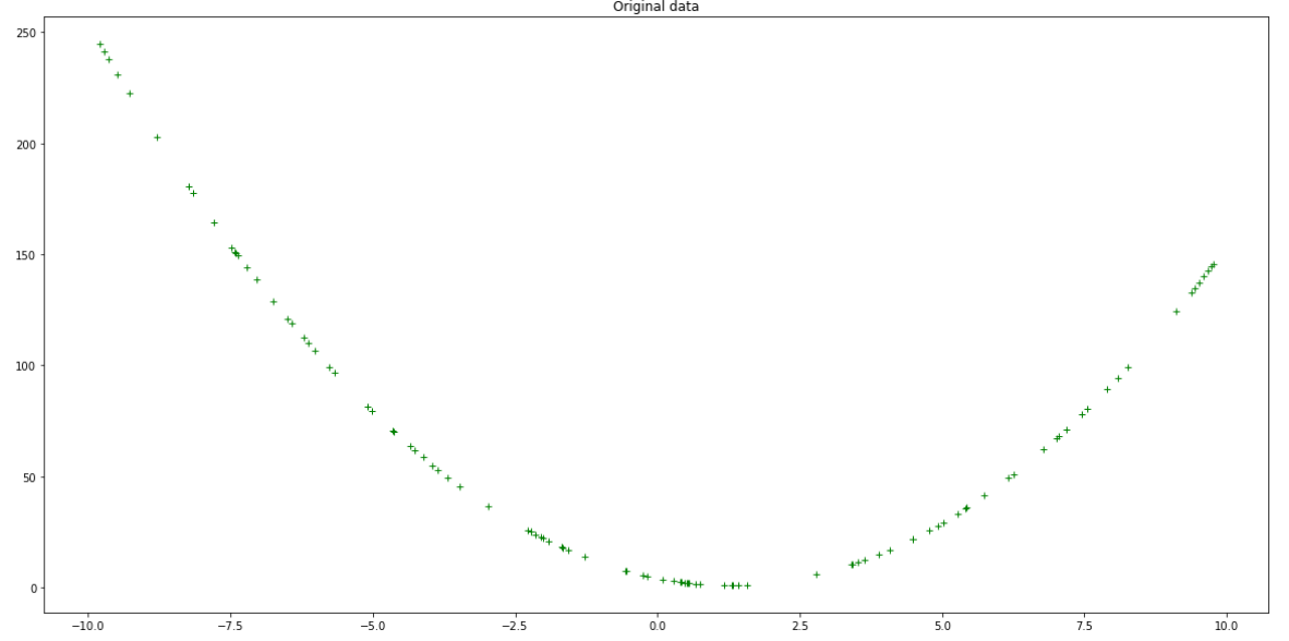
​ Image by Author

Polynomial Regression

We’re specifically looking at polynomial regression here, where the relationship between the independent variable x and the dependent variable y is modeled as an nth degree polynomial in x. Simply put, the coefficients of our second degree polynomial a,b and c will be estimated, evaluated and altered until we can accurately fit a line to the input x data. Gradient descent is the optimization step in this process that alters and improves on the values of these coefficients.

We will now look at how to create and plot such a curve, and then build an initial model to fit to this data, which we will then optimize and improve on using gradient descent. If we can get a model that accurately describes the data, the hope is that it should be able to accurately predict the y values of another set of x values.

We can start be choosing coefficients for a second degree polynomial equation (𝑎𝑥²+𝑏𝑥+𝑐) that will distribute the data we will try to model:

coeffs = [2, -5, 4]

These will be the coefficients for our base/ground truth model we hope to get our predictive model as close as possible to. Next, we need an evaluation function for a second degree polynomial, which, given a set of coefficients and a given input 𝑥 returns the corresponding 𝑦:

def eval_2nd_degree(coeffs, x):
    """
    Function to return the output of evaluating a second degree polynomial,
    given a specific x value.
    
    Args:
        coeffs: List containing the coefficients a,b, and c for the polynomial.
        x: The input x value to the polynomial.
    
    Returns:
        y: The corresponding output y value for the second degree polynomial.
    
    """
    a = (coeffs[0]*(x*x))
    b = coeffs[1]*x
    c = coeffs[2]
    y = a+b+c
    return y
    

We can see it in action when x=3*:*

coeffs = [2, -5, 4]
x=3
eval_2nd_degree(coeffs, x)

7

Creating the data and base model

Define some x data (inputs) we hope to predict y (outputs) of:

import numpy as np
import matplotlib.pyplot as plt

hundred_xs=np.random.uniform(-10,10,100)
print(hundred_xs)

x_y_pairs = []
for x in hundred_xs:
    y  = eval_2nd_degree(coeffs, x)
    x_y_pairs.append((x,y))
    
xs = []
ys = []
for a,b in x_y_pairs:
    xs.append(a)
    ys.append(b)
    
plt.figure(figsize=(20,10))
plt.plot(xs, ys, 'g+')
plt.title('Original data')
plt.show()

​ Curve for polynomial 2x² -5x + 4 = 0 — Author

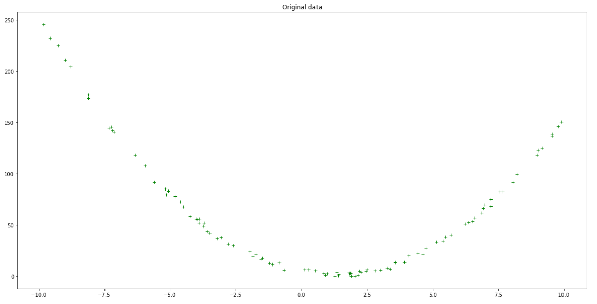
This is good, but we could improve on this by making things more realistic. You can add noise or ‘jitter’ to the values so they can resemble real-world data:

def eval_2nd_degree_jitter(coeffs, x, j):
    """
    Function to return the noisy output of evaluating a second degree polynomial,
    given a specific x value. Output values can be within [y−j,y+j].
    
    Args:
        coeffs: List containing the coefficients a,b, and c for the polynomial.
        x: The input x value to the polynomial.
        j: Jitter parameter, to introduce noise to output y.
    
    Returns:
        y: The corresponding jittered output y value for the second degree polynomial.
    
    """
    a = (coeffs[0]*(x*x))
    b = coeffs[1]*x
    c = coeffs[2]
    y = a+b+c
    print(y)
    
    interval = [y-j, y+j]
    interval_min = interval[0]
    interval_max = interval[1]
    print(f"Should get value in the range {interval_min} - {interval_max}")
    jit_val = random.random() * interval_max      # Generate a random number in range 0 to interval max 
    
    while interval_min > jit_val:                 # While the random jitter value is less than the interval min,
        jit_val = random.random() * interval_max  # it is not in the right range. Re-roll the generator until it 
                                                  # give a number greater than the interval min. 
    
    return jit_val

Test it out:

x=3
j=4
eval_2nd_degree_jitter(coeffs, x, j)

7
Should get value in the range 3 - 116.233537936801398

This updated function will take in the inputs for the second-order polynomial and a jitter value j to add noise to this input, to give us a more realistic output than just a perfect curve:

x_y_pairs = []
for x in hundred_xs:
    y  = eval_2nd_degree_jitter(coeffs, x, j)
    x_y_pairs.append((x,y))
    
xs = []
ys = []
for a,b in x_y_pairs:
    xs.append(a)
    ys.append(b)
    
plt.figure(figsize=(20,10))
plt.plot(xs, ys, 'g+')
plt.title('Original data')
plt.show()

​ Original data with jitter — Author

When we build our predictive model, and optimize it with gradient descent, hopefully we will get as close to these values as possible.

First pass at modelling — try a random model

The first pass at modelling involves generating and storing random coefficients for a second degree polynomial (𝑦=𝑎𝑥² +𝑏𝑥+𝑐). This will be our initial model which will most likely not be that accurate, which we will aim to improve upon until it fits the data well enough.

rand_coeffs = (random.randrange(-10, 10), random.randrange(-10, 10), random.randrange(-10,10))

rand_coeffs

(7, 6, 3)

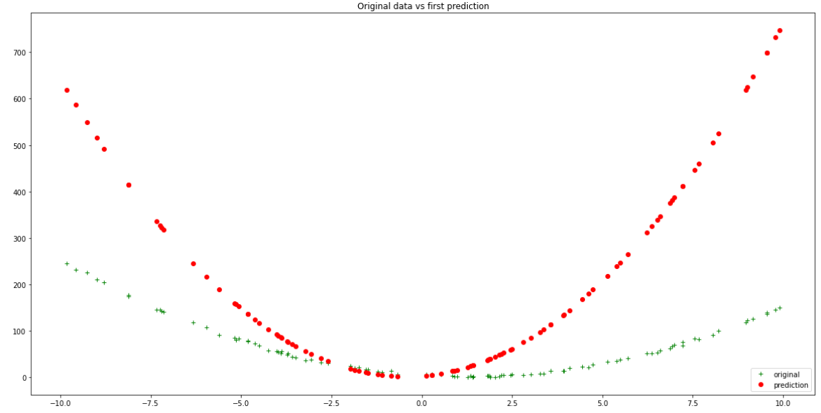
Inspect this model’s accuracy by calculating the predicted output values from your input values:

y_bar = eval_2nd_degree(rand_coeffs, hundred_xs)

plt.figure(figsize=(20,10))
plt.plot(xs, ys, 'g+', label = 'original')
plt.plot(xs, y_bar, 'ro', label='prediction')
plt.title('Original data vs first prediction')
plt.legend(loc="lower right")
plt.show()

​ Original data vs first random prediction — Author

It is evident from the above plot that this new model with random coefficients does not fit our data all that well. To get a quantifiable measure of how incorrect it is, we calculate the Mean Squared Error loss for the model. This is the mean value of the sum of the squared differences between the actual and predicted outputs:

def loss_mse(ys, y_bar):
    """
    Calculates MSE loss.
    
    Args:
        ys: training data labels
        y_bar: prediction labels
    
    Returns: Calculated MSE loss.
    """
    return sum((ys - y_bar)*(ys - y_bar)) / len(ys)
  
  initial_model_loss = loss_mse(ys, y_bar)
  
  initial_model_loss

47922.39790821987

Quite a large number. Let’s now see if we can improve on this fairly high loss metric by optimizing the model with gradient descent.

Gradient Descent and Loss Reduction

We wish to improve our model. Therefore we want to alter its coefficients a, b and c to decrease the error. Therefore we require knowledge about how each coefficient affects the error. This is achieved by calculating the partial derivative of the loss function with respect to each of the individual coefficients.

In this case, we are using MSE as our loss function — this is the function we wish to calculate partial derivatives for:

With output predictions for our model as:

Loss can therefore be reformulated as:

In this specific case, our partial derivatives for that loss function are the following:

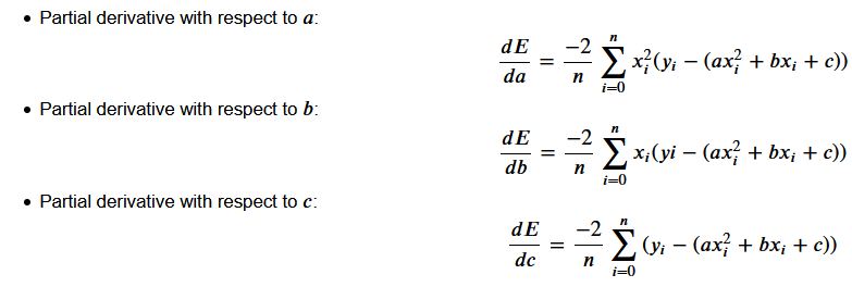
• If you calculate the value of each derivative, you will obtain the gradient for each coefficient.
• These are the values that give you the slope of the loss function with regards to each specific coefficient.
• They indicate whether you should increase or decrease it to reduce the loss, and also by how much it should be safe to do so.

Given coefficients 𝑎, 𝑏 and 𝑐, calculated gradients 𝑔𝑎, 𝑔𝑏 and 𝑔𝑐 and a learning rate 𝑙𝑟, typically one would update the coefficients so that their new, updated values are defined as below:

Once you have applied that new model to the data, your loss should have decreased.

Get that loss down

We need a gradient calculation function which, given a second degree polynomial’s coefficients, as well as a set of inputs 𝑥 and a corresponding set of actual outputs 𝑦 will return the respective gradients for each coefficient.

def calc_gradient_2nd_poly(rand_coeffs, hundred_xs, ys): 
    """
    calculates the gradient for a second degree polynomial.
    
    Args:
        coeffs: a,b and c, for a 2nd degree polynomial [ y = ax^2 + bx + c ]
        inputs_x: x input datapoints
        outputs_y: actual y output points
        
    Returns: Calculated gradients for the 2nd degree polynomial, as a tuple of its parts for a,b,c respectively.
    
    """
    
    a_s = []
    b_s = []
    c_s = []
    
    
    y_bars = eval_2nd_degree(rand_coeffs, hundred_xs)
    
    for x,y,y_bar in list(zip(hundred_xs, ys, y_bars)):    # take tuple of (x datapoint, actual y label, predicted y label)
        x_squared = x**2
        partial_a = x_squared * (y - y_bar)
        a_s.append(partial_a)
        partial_b = x * (y-y_bar)
        b_s.append(partial_b)
        partial_c = (y-y_bar)
        c_s.append(partial_c)
    
    num = [i for i in y_bars]
    n = len(num)
    
    gradient_a = (-2 / n) * sum(a_s)
    gradient_b = (-2 / n) * sum(b_s)
    gradient_c = (-2 / n) * sum(c_s)
    return(gradient_a, gradient_b, gradient_c)   # return calculated gradients as a a tuple of its 3 parts

We’re now going to:

• Use the above function to calculate gradients for our poor-performing random model,
• Adjust the model’s coefficients accordingly,
• Verify that the model’s loss is now smaller — that G.D. has worked!

Let’s set an initial learning rate to experiment with. This should be kept small to avoid the missing the global minimum, but not so small that it takes forever or gets stuck in a local minimum. lr = 0.0001 is a good place to start.

calc_grad = calc_gradient_2nd_poly(rand_coeffs, hundred_xs, ys)

lr = 0.0001
a_new = rand_coeffs[0] - lr * calc_grad[0]
b_new = rand_coeffs[1] - lr * calc_grad[1]
c_new = rand_coeffs[2] - lr * calc_grad[2]

new_model_coeffs = (a_new, b_new, c_new)
print(f"New model coeffs: {new_model_coeffs}")
print("")

#update with these new coeffs:
new_y_bar = eval_2nd_degree(new_model_coeffs, hundred_xs)
updated_model_loss = loss_mse(ys, new_y_bar)

print(f"Now have smaller model loss: {updated_model_loss} vs {original_model_loss}")

New model coeffs: 5.290395171471687 5.903335222089396 2.9704266522693037Now have smaller model loss: 23402.14716735533 vs 47922.39790821987

Visualize this improvement by plotting the training data, original random model and updated lower-loss model together:

plt.figure(figsize=(20,10))
plt.plot(xs, ys, 'g+', label = 'original model')
plt.plot(xs, y_bar, 'ro', label = 'first prediction')
plt.plot(xs, new_y_bar, 'b.', label = 'updated prediction')
plt.title('Original model vs 1st prediction vs updated prediction with lower loss')
plt.legend(loc="lower right")
plt.show()

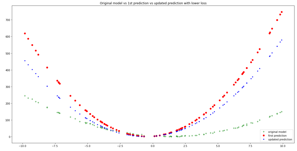
​ Improved accuracy after one iteration of gradient descent - Author

Iterative Gradient Descent over many epochs

We’re almost ready. The last step will be to perform gradient descent iteratively over a number of epochs (cycles or iterations.) With every epoch we hope to see an improvement in the from of lowered loss, and better model-fitting to the original data.

Let’s improve on the calc_gradient_2nd_poly function from above, to make it more usable for an iterative gradient descent process:

def calc_gradient_2nd_poly_for_GD(coeffs, inputs_x, outputs_y, lr): 
    """
    calculates the gradient for a second degree polynomial.
    
    Args:
        coeffs: a,b and c, for a 2nd degree polynomial [ y = ax^2 + bx + c ]
        inputs_x: x input datapoints
        outputs_y: actual y output points
        lr: learning rate
        
    Returns: Calculated gradients for the 2nd degree polynomial, as a tuple of its parts for a,b,c respectively.
    
    """
    a_s = []
    b_s = []
    c_s = []
        
    y_bars = eval_2nd_degree(coeffs, inputs_x)

    for x,y,y_bar in list(zip(inputs_x, outputs_y, y_bars)):    # take tuple of (x datapoint, actual y label, predicted y label)
        x_squared = x**2        
        partial_a = x_squared * (y - y_bar)
        a_s.append(partial_a)
        partial_b = x * (y-y_bar)
        b_s.append(partial_b)
        partial_c = (y-y_bar)
        c_s.append(partial_c)
    
    num = [i for i in y_bars]
    n = len(num)
    
    gradient_a = (-2 / n) * sum(a_s)
    gradient_b = (-2 / n) * sum(b_s)
    gradient_c = (-2 / n) * sum(c_s)


    a_new = coeffs[0] - lr * gradient_a
    b_new = coeffs[1] - lr * gradient_b
    c_new = coeffs[2] - lr * gradient_c
    
    new_model_coeffs = (a_new, b_new, c_new)
    
    #update with these new coeffs:
    new_y_bar = eval_2nd_degree(new_model_coeffs, inputs_x)
    
    updated_model_loss = loss_mse(outputs_y, new_y_bar)
    return updated_model_loss, new_model_coeffs, new_y_bar

This will be called as part of the gradient_descent function:

def gradient_descent(epochs, lr):
    """
    Perform gradient descent for a second degree polynomial.
    
    Args:
        epochs: number of iterations to perform of finding new coefficients and updatingt loss. 
        lr: specified learning rate
        
    Returns: Tuple containing (updated_model_loss, new_model_coeffs, new_y_bar predictions, saved loss updates)
    
    """
    losses = []
    rand_coeffs_to_test = rand_coeffs
    for i in range(epochs):
        loss = calc_gradient_2nd_poly_for_GD(rand_coeffs_to_test, hundred_xs, ys, lr)
        rand_coeffs_to_test = loss[1]
        losses.append(loss[0])
    print(losses)
    return loss[0], loss[1], loss[2], losses  #(updated_model_loss, new_model_coeffs, new_y_bar, saved loss updates)

Finally, let’s train for 1500 epochs and see if our model has learned anything:

GD = gradient_descent(1500, 0.0001)

plt.figure(figsize=(20,10))
plt.plot(xs, ys, 'g+', label = 'original')
plt.plot(xs, GD[2], 'b.', label = 'final_prediction')
plt.title('Original vs Final prediction after Gradient Descent')
plt.legend(loc="lower right")
plt.show()

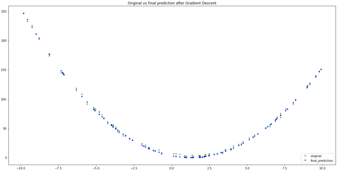
​ Quite close to the original data! — Author

This trained model is showing vast improvements after it’s full training cycle. We can examine further by inspecting its final predicted coefficients a,b and c:

print(f"Final Coefficients predicted: {GD[1]}")
print(f"Original Coefficients: {coeffs}")

Final Coefficients predicted: (2.0133237089326155, -4.9936501002139275, 3.1596042252126195)
Original Coefficients: [2, -5, 4]

Not too far off! A big improvement over the initial random model. Looking at the plot of the loss reduction over training offers further insights:

plt.figure(figsize=(20,10))
plt.plot(GD[3], 'b-', label = 'loss')
plt.title('Loss over 1500 iterations')
plt.legend(loc="lower right")
plt.xlabel('Iterations')
plt.ylabel('MSE')
plt.show()

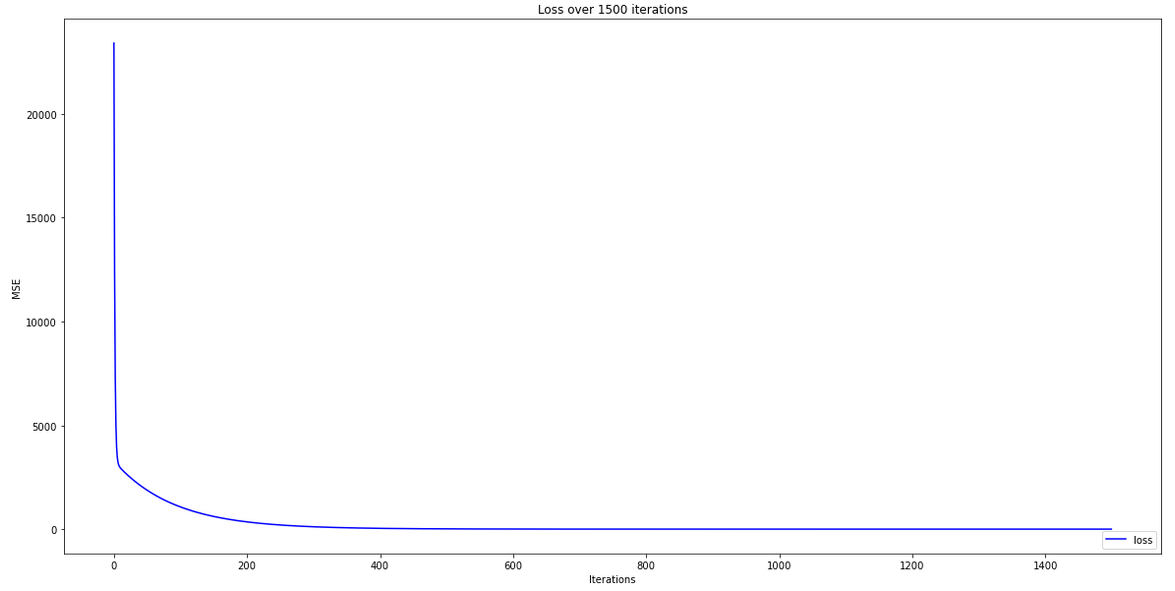
​ Loss reduction over epochs — Author

We observe that the model loss reached close to zero, to give us our more accurate coefficients. We can also see there was no major improvement in loss after about 400 epochs — definitely no need for 1500 epochs. An alternative strategy would be to add some kind of condition to the training step that stops training when a certain minimum loss threshold has been reached. This would prevent excessive training and potential over-fitting for the model.

I hope you enjoyed this dive into gradient descent for polynomial regression. Certain concepts can be daunting to understand at first glance, but over time we become familiar with the ‘nuts and bolts’ of a problem if we stick at it long enough. I found this was certainly the case for me with this exercise, and feel it was a worthwhile learning experience overall.